
Everyone declared this the era of agents, and for once the hype has a real engine under it. We run one in production. A continuous stream of developer requests comes in; the agent reads each brief and answers with the people from our seventeen-person bench who can actually do the work, under real constraints: stack, seniority, rate, availability. Matching is exactly the kind of job you hand an agent. High volume, hard conditions, expensive in human hours, and visible to a client when it is wrong.
The first version used plain vector search. It was fluent, fast, and confidently wrong. Ask it for a React Native engineer who had shipped a payments flow, and it returned strong, well-rounded generalists while burying the one person whose history literally said React Native and Stripe. The meaning was close. The exact words that mattered got averaged into a smooth blur.
The model was never the problem. The retrieval was. An agent is only as smart as its search, and the search is the part of RAG that vendor demos skip. It is where most production systems quietly fail.
The embedding model is the easy part. What breaks in production is everything around it.
Here is the path from plain vectors to hybrid search, told through the system we actually run, with the reasoning behind each piece. There is a fusion demo in the middle you can tune yourself.
What RAG actually fixes
A language model is good at phrasing and bad at knowing your private facts. It has never seen our team's employment history, and it never will. When you ask it something outside its training, it does not stop. It produces a confident, plausible answer that happens to be invented.
RAG, retrieval-augmented generation, turns a closed-book exam into an open-book one. Before the model answers, you search your own data for the passages that matter and hand them over with the question. The model stops guessing and starts summarizing facts you retrieved. The quality of the answer is now capped by the quality of the search, not the size of the model. That is the whole reason retrieval deserves real engineering attention instead of a library call you paste once and forget.
How vectors find meaning
To search by meaning instead of exact words, you turn text into a dense vector, a long list of numbers that encodes what a passage is about. Similar meanings land near each other in that space. A query becomes a vector too, and the search is simply this: find the stored vectors nearest to this one.
The naive way to do that is to compare the query against every record. With a few hundred rows that is fine. With millions it is a linear scan that pins a CPU and blows your latency budget. So a vector database builds an index that avoids looking at almost everything.
The idea behind that index is older than vector search. In 1967 the psychologist Stanley Milgram handed packets to people in Nebraska and asked each one to forward the packet to whoever they knew who seemed socially closer to a stranger in Boston. The packets that made it took about six hops. Nobody held a map of the whole country. Each person made one good local decision and passed it on. That is the small-world effect, the same intuition behind six degrees of separation, and it is almost exactly how a modern vector index finds a neighbor.
HNSW, Hierarchical Navigable Small World, is a stack of those small-world graphs. The clean way to picture it is layers of roads. The top layer has a few long-distance routes that cross the whole map in one hop. The middle layer adds regional connections. The bottom layer is every local street, where the records actually live. A search starts at the top, takes a couple of long hops to reach the right region, drops a layer, refines, drops again, and arrives at the right neighborhood in a few dozen steps instead of millions of comparisons. Like Milgram's packets, it never looks at the whole map. It just keeps moving to a closer neighbor.
We never wrote that index by hand. Qdrant builds and maintains the HNSW graph itself, which matters more than it sounds, and I will come back to it.
Where pure vector search quietly fails
Dense vectors are good at meaning and bad at exact identifiers. They understand that mobile developer and iOS engineer are related. They are much weaker when the thing that matters is one precise token: a specific framework, a version number, a client name, the exact title of a certificate.
That was our matcher's failure. A request for React Native is not a request for the general vibe of mobile work. It is a request for that exact skill, and a dense vector blends it into the surrounding meaning until it stops being decisive. The same goes for a brand the client names directly, an error code in a support ticket, or a niche library only one person on the team has touched. The detail that should win the match is exactly the detail dense search smooths away.
Dense vectors understand what you mean. Sparse vectors remember what you said.
Sparse vectors and the return of the exact match
The answer is older than embeddings. It is the inverted index, the structure search engines have used for decades to map each word to the documents that contain it. The classic scoring on top of it is BM25, born in the Okapi search system in the 1990s; the BM is just best matching, formula number twenty-five, and it is still a strong baseline thirty years later. In vector terms that is a sparse vector: mostly zeros, with weight on the specific terms that actually appear.
Modern sparse models are smarter than raw keyword counts. We use SPLADE, which stands for sparse lexical and expansion. It runs the text through a BERT head that does two jobs at once: it weights the words that carry meaning, and it quietly expands them to close relatives, so a passage about a car also lights up vehicle and automobile while the stopwords fade. You get the precision of keyword search without its brittleness. An exact hit on React Native still fires when the text only says RN. The expansion is also the honest tradeoff: a learned model can spread weight onto neighbors you never asked for. If your domain punishes any drift at all, serial numbers, legal citations, part codes, plain BM25 is the safer sparse side. For skills and job titles the coverage wins, and the fusion weighting keeps it disciplined. Sparse search catches the tokens dense search blurs, which is the half we were missing.
Hybrid search: run both, fuse the rankings
Hybrid search is the obvious move once you can name the two failure modes, and you do not have to take my word for the payoff. When Anthropic published its contextual retrieval work, the version that paired embeddings with a lexical BM25 signal cut failed retrievals by about 49 percent, and adding a reranking step took it to about 67 percent. Their pipeline also prepends a short context to each chunk, so read those numbers as the shape of the win rather than a guarantee. The exact-token half of search is not a rounding error. It is most of the gap. To be fair, the gain is not universal: on a narrow corpus with one uniform vocabulary, dense search alone often saturates and the sparse side adds little. The win shows up where the vocabulary is wide and the queries hang on exact tokens, which is exactly what job briefs and CVs look like.
So you run the dense search for meaning and the sparse search for exact terms, in parallel, then merge the two ranked lists into one.
The merge is the interesting part, because the two searches produce scores on completely different scales. You cannot just add them. The standard method is Reciprocal Rank Fusion. It ignores the raw scores and looks only at position: something ranked first by either search gets a strong boost, and items that rank well in both rise to the top. The 60 in our setup is not a number we picked. It comes from a 2009 paper by Cormack and colleagues, who were fusing search rankings and found that 60 was the value that let agreement between the searches win without letting either one's top result dominate. Almost everyone still uses 60, including us. The one number we did choose is the weight.
One aside, since people ask. RRF is not the only way to fuse. Qdrant also offers DBSF, which normalizes the two score distributions instead of throwing the scores away. That works best when the scores are comparable to begin with. Ours are not: bounded cosine on one side, unbounded sparse sums on the other, and normalizing apples against oranges can let one list quietly dominate. RRF does not look at the scores at all, which is exactly why we trust it here.
Two numbers in that fusion are worth calling out. We use the standard constant of 60, and we weight the sparse list twice as heavily as the dense one. That weighting is a product decision, not a default. For matching a person to a job, an exact skill match should outrank a general semantic resemblance, so the exact-term side gets the louder vote.
You can feel the effect yourself. Below is the same five candidates our matcher might see for that React Native and Stripe brief. Dense search ranks the smooth generalists first. Sparse search ranks the exact match first. Drag the weight and watch where the fused result lands.
Dense ranking (meaning)
Sparse ranking (exact terms)
Fused result · RRF
The moment we shipped hybrid search with that weighting, the person whose history actually said React Native and Stripe came back first. Same data, same model, different retrieval.
Why Qdrant, and when it is the wrong call
We did not start with strong opinions about the database. We ended up on Qdrant because of what hybrid search needs in production, and the comparison is worth making honestly.
Four things decided it for us.
First, hybrid lives in one place. A single Qdrant collection holds both the dense vector, through HNSW, and the sparse vector, through an inverted index, and fuses them in one query. We did not stand up Postgres for the relational side and Elasticsearch for the keyword side and then write glue to reconcile two systems.
Second, the index manages itself. With pgvector you create the HNSW index by hand in SQL and own its tuning and maintenance. Qdrant decides for you: small collections are scanned directly because that is faster, and as the data grows it builds the graph. One less thing to babysit.
Third, filtering is built into the search, not bolted on after it. Our matcher filters constantly: only these section types, only this person, the equivalent of find the passage about a skill, but only inside employment history. And filters are genuinely hard for a graph index. The greedy walk assumes it can always step to a closer neighbor; a selective filter knocks most nodes out, the walk lands in a pocket where every neighbor is excluded, and it stops early, convinced it is done. No error, just quietly worse results. The lazy alternative, fetching nearest neighbors first and filtering after, is no better: a selective filter throws away almost the whole page you just paid for. Qdrant plans around both. It applies the filter while it walks the graph, leaning on payload indexes over the fields you filter by, switches strategy when a filter gets very selective, and since version 1.16 can hop through excluded nodes to their still-valid neighbors, an idea called ACORN, so the walk crosses dead zones instead of stalling in them. For a system whose whole job is search plus conditions, this one property carried the decision.
Fourth, it stays out of the way operationally. Qdrant is one service, written in Rust, and it supports quantization to compress vectors and save memory when you need it. Binary quantization cuts what the vectors themselves occupy by roughly thirty times, with an oversample-and-rescore pass to hold recall. One honest footnote on that headline: the graph structure on top does not compress, so the total memory bill shrinks less than thirty times. We have not needed any of it at the size we run, and that is the point: the capability is there for later, not a cost now.
None of this makes pgvector a mistake. If you already run Postgres, you are under a few million vectors, and you need transactional consistency across your relational data and your vectors in a single query, pgvector is the pragmatic choice and one fewer system to operate. We are not guessing about that side either. Alex Tkachenko, a full-stack engineer on our team, keeps a movie recommendation service on pgvector, public at github.com/BenderBRodrigez/fastapi-movies. Each film carries a 768-dimensional embedding as an ordinary column on the movie row, a user's taste profile is computed as the SQL average of the embeddings in their catalog, and recommendations are one ORDER BY on cosine distance away. Vectors living inside the relational model, aggregated with plain SQL in one transactional query, is the thing a separate vector database cannot give you. At catalog scale it does not even need a vector index; Postgres scans and it is fine. The ceiling moves, too: the pgvectorscale extension adds a disk-based DiskANN index that carries Postgres into the tens of millions of vectors. The honest rule is to match the database to the job, and on our own team the rule split both ways: hybrid retrieval under hard filters went to Qdrant, and the recommender that lives next to its relational data stayed in Postgres.
The managed names most teams reach for first are Pinecone and Weaviate, and both do hybrid too. Pinecone is the least operational of any of them, fully serverless, but it is closed and your vectors live on someone else's infrastructure, a non-starter the moment the data cannot leave the building. Weaviate is the closest open alternative and a fair pick. We landed on Qdrant for the filtered traversal and the quantization, and because it self-hosts next to our own data, which is the constraint most real work shows up with.
Read the code, run the search
This is not a hypothetical. The whole service is open: the repository is public at github.com/2mc-org/cv-matcher-api. The hybrid search this article describes is one file. The collection holds a named dense vector and a named sparse vector, the query issues two prefetch branches, and the fusion is a single Reciprocal Rank Fusion call with k set to 60 and the sparse list weighted at 2.0. It is about forty lines. The interesting work was never the code. It was deciding what the retrieval had to do.
And it runs. A live version sits at cv-matcher.2muchcoffee.com. Tell it a role in plain language and it answers with a ranked shortlist, each name backed by the lines from a real history that earned the match. Ask it something vague and it asks for the role instead of inventing one. The hybrid retrieval in this article is the layer under that conversation.
The chunking is the same kind of boring on purpose. A CV is not prose, it is a small database wearing a document costume: a title, a skill list, a dated job history, certificates. So we never chunk by token count or semantic drift. We cut along the structure, one point per section, one per job, one per certificate. Run a generic semantic chunker over a CV and it reads the jump between two jobs as a topic change and slices the timeline into confetti. The structure was already the chunking. We just respected it.
What this looks like in production
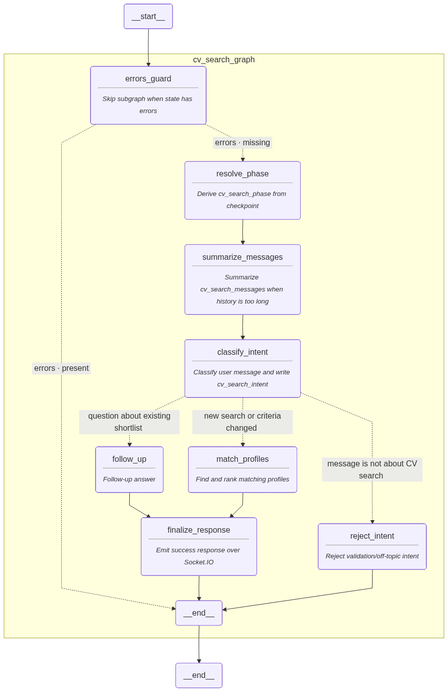
Retrieval is not the end of our pipeline. The ranked list of people feeds the rest of the agent, orchestrated with LangGraph, which drafts a first-pass response, with durable state in Postgres so a long run survives a restart. The agent is only as good as what retrieval hands it. Give it the well-rounded wrong people and it writes a confident, wrong draft. Give it the right match and the rest of the system has something true to work with.
Hybrid is two stages, dense and sparse. There is a third we have not needed yet: a reranker. A cross-encoder, or a late-interaction model like ColBERT, re-reads the query against each top candidate and reorders them, slower but sharper. That is the step that took Anthropic's number from 49 to 67 percent. At seventeen people it is overkill. At seventeen thousand documents it is the first thing I would add. Knowing which stage you actually need is the job.
It is tempting in 2026 to skip all of this and pour everything into one giant context window. The models hold a million tokens now, so why retrieve at all? Because they do not really read the middle. Researchers named it lost in the middle: a fact buried in the center of a long context is far more likely to be ignored than the same fact at the start or the end. A bigger window does not replace retrieval. It just gives you a longer place to lose the thing that mattered.
That is the lesson under all of this, and it is the one I keep relearning. The embedding model and the agent are the parts everyone talks about. The retrieval architecture, the chunking, the fusion, the filtering, the choice of index, is the part that decides whether the thing works when it is no longer a demo.
What 2muchcoffee covers
Our AI engineering team builds production RAG and AI systems the way we built this one: the unglamorous retrieval layer first, because that is what decides whether the output can be trusted. If you have a RAG prototype that demos well and returns confident, slightly wrong answers, the fix is usually not a bigger model. It is the search underneath. The plain path to talk it through is the AI work we do.
One concrete action
Before you reach for a bigger model, run one test on your own RAG. Pick an exact identifier you know is in your data, a specific framework, a product name, a part number, and search for it. If the passage that contains it does not come back at or near the top, you do not have a model problem. You have a sparse problem, and hybrid search is the fix. Start there.


